Notes for Machine Learning Yearning-Draft
从10月份开始到11月份,前后共计花了15天的时间阅读;在阅读过程中,就书中内容进行了摘录和部分扩展阅读记录,供大家参考
原书可以在这里下载:Machine Learning Yearning-Draft
需要笔记PDF版本的,可以在这里下载:Notes for Machine Learning Yearning-Draft
Notes for Machine Learning Yearning-Draft
Overview
4. Scale drives machine learning progress
- Data availability
- Computational scale
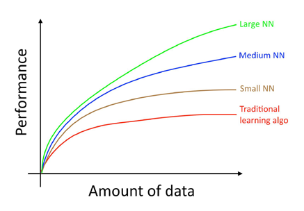
Many other details such as neural network architecture are also important, and there has been much innovation here. But one of the more reliable ways to improve an algorithm’s performance today is still to (i) train a bigger network and (ii) get more data.
Setting up development and test sets
5. Your development and test sets
Before the modern era of big data, it was a common rule in machine learning to use a random 70%/30% split to form your training and test sets. This practice can work, but it’s a bad idea in more and more applications where the training distribution is different from the distribution you ultimately care about.
- Training set — Which you run your learning algorithm on.
- Dev (development) set — Which you use to tune parameters, select features, and make other decisions regarding the learning algorithm. Sometimes also called the hold-out cross validation set.
- Test set — which you use to evaluate the performance of the algorithm, but not to make any decisions regarding what learning algorithm or parameters to use.
In other words, the purpose of the dev and test sets are to direct your team toward the most important changes to make to the machine learning system.
Try to pick test examples that reflect what you ultimately want to perform well on, rather than whatever data
you happen to have for training.
7. How large do the dev/test sets need to be?
Dev sets with sizes from 1,000 to 10,000 examples are common. With 10,000 examples, you will have a good chance of detecting an improvement of 0.1%.
One popular heuristic had been to use 30% of your data for your test set. This works well when you have a modest number of examples—say 100 to 10,000 examples. But in the era of big data where we now have machine learning problems with sometimes more than a billion examples, the fraction of data allocated to dev/test sets has been shrinking, even as the absolute number of examples in the dev/test sets has been growing. There is no need to have excessively large dev/test sets beyond what is needed to evaluate the performance of your algorithms.
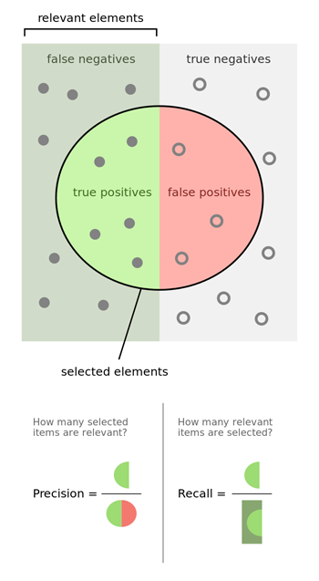
8. Establish a single-number evaluation metric for your team to optimize
Classification accuracy is an example of a single-number evaluation metric. In contrast, Precision and Recall is not a single-number evaluation metric.
Having a single-number evaluation metric such as accuracy allows you to sort all your models according to their performance on this metric, and quickly decide what is working best.
If you really care about both Precision and Recall, I recommend using one of the standard ways to combine them into a single number. Alternatively, you can compute the “F1 score”, which is a modified way of computing their average, and works better than simply taking the mean.
$$ F_1 = \big(\frac{recall^{-1}+precision^{-1}}{2}\big)^{-1} = 2\cdot\frac{precision\cdot{recall}}{precision+recall} $$
Reference: https://en.wikipedia.org/wiki/F1_score
Having a single-number evaluation metric speeds up your ability to make a decision when you are selecting among a large number of classifiers. It gives a clear preference ranking among all of them, and therefore a clear direction for progress.
Taking an average or weighted average is one of the most common ways to combine multiple metrics into one.
9. Optimizing and satisficing metrics
If you are trading off N different criteria, you might consider setting N-1 of the criteria as “satisficing” metrics. Then define the final one as the “optimizing” metric.
10. Having a dev set and metric speeds up iterations
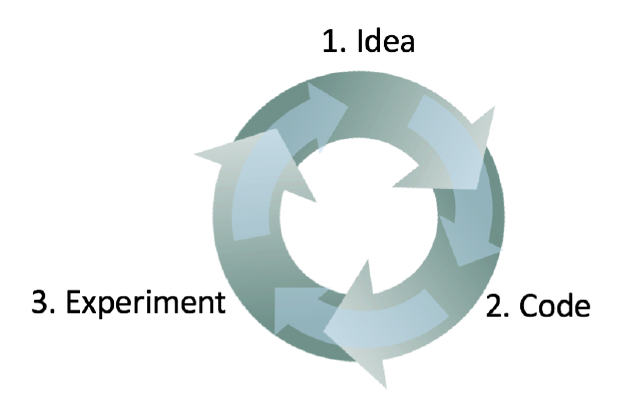
This is an iterative process. The faster you can go round this loop, the faster you will make progress. This is why having dev/test sets and a metric are important: Each time you try an idea, measuring your idea’s performance on the dev set lets you quickly decide if you’re heading in the right direction.
Having a dev set and metric allows you to very quickly detect which ideas are successfully giving you small (or large) improvements, and therefore lets you quickly decide what ideas to keep refining, and which ones to discard.
11. When to change dev/test sets and metrics
It is better to come up with something imperfect and get going quickly, rather than overthink this. But this one week timeline does not apply to mature applications.
There are three main possible causes of the dev set/metric incorrectly rating classifier A higher:
The actual distribution you need to do well on is different from the dev/test sets.
You have overfit to the dev set.
- If you find that your dev set performance is much better than your test set performance, it is a sign that you have overfit to the dev set. In this case, get a fresh dev set.
- But do not use the test set to make any decisions regarding the algorithm, including whether to roll back to the previous week’s system. If you do so, you will start to overfit to the test set, and can no longer count on it to give a completely unbiased estimate of your system’s performance.
The metric is measuring something other than what the project needs to optimize.
Basic Error Analysis
13. Build your first system quickly, then iterate
It is even harder if you are not an expert in the application area. So don’t start off trying to design and build the perfect system. Instead, build and train a basic system quickly—perhaps in just a few days.
14. Error analysis: Look at dev set examples to evaluate ideas
I recommend that you first estimate how much it will actually improve the system’s accuracy. Then you can more rationally decide if this is worth the month of development time, or if you’re better off using that time on other tasks.
The process of looking at misclassified examples is called error analysis.
Error analysis can often help you figure out how promising different directions are.
It often feels more exciting to just jump in and implement some idea, rather than question if the idea is worth the time investment. This is a common mistake: It might result in your team spending a month only to realize afterward that it resulted in little benefit.
Error Analysis refers to the process of examining dev set examples that your algorithm misclassified, so that you can understand the underlying causes of the errors. This can help you prioritize projects and inspire new directions.
15. Evaluating multiple ideas in parallel during error analysis
The most helpful error categories will be ones that you have an idea for improving.
Error analysis does not produce a rigid mathematical formula that tells you what the highest priority task should be. You also have to take into account how much progress you expect to make on different categories and the amount of work needed to tackle each one.
16. Cleaning up mislabeled dev and test set examples
During error analysis, you might notice that some examples in your dev set are mislabeled.
It is not uncommon to start off tolerating some mislabeled dev/test set examples, only later to change your mind as your system improves so that the fraction of mislabeled examples grows relative to the total set of errors.
If you decide to improve the label quality, consider double-checking both the labels of examples that your system misclassified as well as labels of examples it correctly classified.
17. If you have a large dev set, split it into two subsets, only one of which you look at
Why do we explicitly separate the dev set into Eyeball and Blackbox dev sets? Since you will gain intuition about the examples in the Eyeball dev set, you will start to overfit the Eyeball dev set faster. If you see the performance on the Eyeball dev set improving much more rapidly than the performance on the Blackbox dev set, you have overfit the Eyeball dev set.In this case, you might need to discard it and find a new Eyeball dev set by moving moreexamples from the Blackbox dev set into the Eyeball dev set or by acquiring new labeled
data.
Explicitly splitting your dev set into Eyeball and Blackbox dev sets allows you to tell when your manual error analysis process is causing you to overfit the Eyeball portion of your data.
18. How big should the Eyeball and Blackbox dev sets be?
The lower your classifier’s error rate, the larger your Eyeball dev set needs to be in order to get a large enough set of errors to analyze.
If you are working on a task that even humans cannot do well, then the exercise of examining an Eyeball dev set will not be as helpful because it is harder to figure out why the algorithm didn’t classify an example correctly. In this case, you might omit having an Eyeball dev set.
We previously said that dev sets of around 1,000-10,000 examples are common. To refine that statement, a Blackbox dev set of 1,000-10,000 examples will often give you enough data to tune hyperparameters and select among models, though there is little harm in having even more data. A Blackbox dev set of 100 would be small but still useful.
If you have a small dev set, then you might not have enough data to split into Eyeball and Blackbox dev sets that are both large enough to serve their purposes. Instead, your entire dev set might have to be used as the Eyeball dev set.
If you only have an Eyeball dev set, you can perform error analyses, model selection and hyperparameter tuning all on that set. The downside of having only an Eyeball dev set is that the risk of overfitting the dev set is greater.
Bias and Variance
20. Bias and Variance: The two big sources of error
There are two major sources of error in machine learning: bias (the algorithm’s error rate on the training set) and variance (how much worse the algorithm does on the dev).
When your error metric is mean squared error, you can write down formulas specifying these two quantities, and prove that Total Error = Bias + Variance. But for our purposes of deciding how to make progress on an ML problem, the more informal definition of bias and variance given here will suffice.
21. Examples of Bias and Variance
The classifier has very low training error, but it is failing to generalize to the dev set. This is also called overfitting.
This classifier therefore has high bias , but low variance. We say that this algorithm is underfitting.
This classifier has high bias and high
variance. The overfitting/underfitting terminology is hard to apply here since the classifier is simultaneously overfitting and underfitting.
22. Comparing to the optimal error rate
- Optimal error rate(unavoidable bias)
- Avoidable bias: This is calculated as the difference between the training error and the optimal error rate. If this number is negative, you are doing better on the training set than the optimal error rate. This means you are overfitting on the training set, and the algorithm has over-memorized the training set.
You should focus on variance reduction methods rather than on further bias reduction methods. - Variance: The difference between the dev error and the training error.
$$ Bias = Optimal\ error\ rate(unavoidable\ bias) + Avoidable\ bias $$
In theory, we can always reduce variance to nearly zero by training on a massive training set. Thus, all variance is “avoidable” with a sufficiently large dataset, so there is no such thing as “unavoidable variance”.
Knowing the optimal error rate is helpful for guiding our next steps. In statistics, the optimal error rate is also called Bayes error rate, or Bayes rate.
23. Addressing Bias and Variance
- If you have high avoidable bias, increase the size of your model (for example, increase the size of your neural network by adding layers/neurons).
- If you have high variance, add data to your training set.
If you are able to increase the neural network size and increase training data without limit, it is possible to do very well on many learning problems.
In practice, increasing the size of your model will eventually cause you to run into computational problems because training very large models is slow. You might also exhaust your ability to acquire more training data.
The results of trying new architectures are less predictable than the simple formula of increasing the model size and adding data.
Increasing the model size generally reduces bias, but it might also increase variance and the risk of overfitting. However, this overfitting problem usually arises only when you are not using regularization. If you include a well-designed regularization method, then you can usually safely increase the size of the model without increasing overfitting.
The only reason to avoid using a bigger model is the increased computational cost.
24. Bias vs. Variance tradeoff
Of the changes you could make to most learning algorithms, there are some that reduce bias errors but at the cost of increasing variance, and vice versa. This creates a “trade off” between bias and variance.
Alternatively, adding regularization generally increases bias but reduces variance. By adding training data, you can also usually reduce variance without affecting bias.
25. Techniques for reducing avoidable bias
- Increase the model size (such as number of neurons/layers): If you find that this increases variance, then use regularization, which will usually eliminate the increase in variance.
- Modify input features based on insights from error analysis: In theory, adding more features could increase the variance; but if you find this to be the case, then use regularization, which will usually eliminate the increase in variance.
- Reduce or eliminate regularization (L2 regularization, L1 regularization, dropout): This will reduce avoidable bias, but increase variance.
- Modify model architecture (such as neural network architecture) so that it is more suitable for your problem: This technique can affect both bias and variance.
One method that is not helpful:
- Add more training data : This technique helps with variance problems, but it usually has no significant effect on bias.
26. Error analysis on the training set
Similar to the dev set error analysis, you can count the errors in different categories.
27. Techniques for reducing variance
- Add more training data
- Add regularization (L2 regularization, L1 regularization, dropout): This technique reduces variance but increases bias.
- Add early stopping (i.e., stop gradient descent early, based on dev set error): This technique reduces variance but increases bias. Early stopping behaves a lot like regularization methods, and some authors call it a regularization technique.
- Feature selection to decrease number/type of input features: This technique might help with variance problems, but it might also increase bias.
- Decrease the model size (such as number of neurons/layers): Use with caution. This technique could decrease variance, while possibly increasing bias. However, I don’t recommend this technique for addressing variance. Adding regularization usually gives better classification performance. The advantage of reducing the model size is reducing your computational cost and thus speeding up how quickly you can train models. If speeding up model training is useful, then by all means consider decreasing the model size. But if your goal is to reduce variance, and you are not concerned about the computational cost, consider adding regularization instead.
- Modify input features based on insights from error analysis: These new features could help with both bias and variance. In theory, adding more features could increase the variance; but if you find this to be the case, then use regularization, which will usually eliminate the increase in variance.
- Modify model architecture (such as neural network architecture) so that it is more suitable for your problem: This technique can affect both bias and variance.
Learning curves
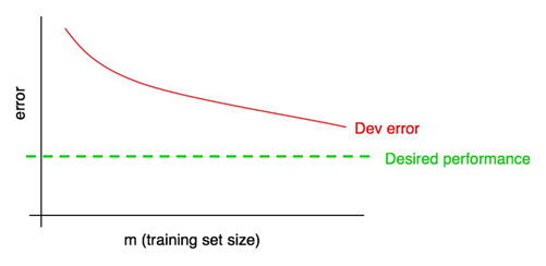
28. Diagnosing bias and variance: Learning curves
A learning curve plots your dev set error against the number of training examples.
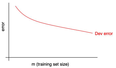
As the training set size increases, the dev set error should decrease.
Add the desired level of performance to your learning curve:
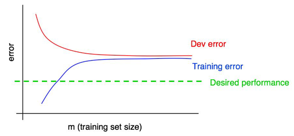
29. Plotting training error
Your training set error usually increases as the training set size grows.

30. Interpreting learning curves: High bias
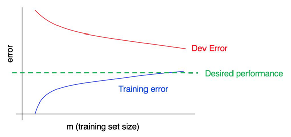
31. Interpreting learning curves: Other cases
The bias is small, but the variance is large. Adding more training data will probably help close the gap between dev error and training error.
You have significant bias and significant variance. You will have to find a way to reduce both bias and
variance in your algorithm.

32. Plotting learning curves
If the noise in the training curve makes it hard to see the true trends, here are two solutions:
- Instead of training just one model on 10 examples, instead select several (say 3-10) different randomly chosen training sets of 10 examples by sampling with replacement 10 from your original set of 100. Train a different model on each of these, and compute the training and dev set error of each of the resulting models. Compute and plot the average training error and average dev set error.
- If your training set is skewed towards one class, or if it has many classes, choose a “balanced” subset instead of 10 training examples at random out of the set of 100.
I would not bother with either of these techniques unless you have already tried plotting learning curves and concluded that the curves are too noisy to see the underlying trends. If your training set is large—say over 10,000 examples—and your class distribution is not very skewed, you probably won’t need these techniques.
Finally, plotting a learning curve may be computationally expensive: For example, you might have to train ten models with 1,000, then 2,000, all the way up to 10,000 examples. Training models with small datasets is much faster than training models with large datasets. Thus, instead of evenly spacing out the training set sizes on a linear scale as above, you might train models with 1,000, 2,000, 4,000, 6,000, and 10,000 examples. This should still give you a clear sense of the trends in the learning curves. Of course, this technique is relevant only if the computational cost of training all the additional models is significant.
Comparing to human-level performance
33. Why we compare to human-level performance
Further, there are several reasons building an ML system is easier if you are trying to do a task that people can do well:
- Ease of obtaining data from human labelers.
- Error analysis can draw on human intuition.
- Use human-level performance to estimate the optimal error rate and also set a “desired error rate”.
There are some tasks that even humans aren’t good at.
- It is harder to obtain labels.
- Human intuition is harder to count on.
- It is hard to know what the optimal error rate and reasonable desired error rate is.
Training and testing on different distributions
36. When you should train and test on different distributions
Most of the academic literature on machine learning assumes that the training set, dev set and test set all come from the same distribution. In the early days of machine learning, data 11 was scarce. We usually only had one dataset drawn from some probability distribution. So we would randomly split that data into train/dev/test sets, and the assumption that all the data was coming from the same source was usually satisfied.
There is some academic research on training and testing on different distributions. Examples include “domain adaptation”, “transfer learning” and “multitask learning”. But there is still a huge gap between theory and practice.
37. How to decide whether to use all your data
When using earlier generations of learning algorithms (such as hand-designed computer vision features, followed by a simple linear classifier) there was a real risk that merging both types of data would cause you to perform worse.
But in the modern era of powerful, flexible learning algorithms—such as large neural networks—this risk has greatly diminished.
Adding the additional data has the following effects:
- It gives your neural network more examples of what cats do/do not look like.
- It forces the neural network to expend some of its capacity to learn about different properties. Theoretically, this could hurt your algorithms’ performance.
If you think you have data that has no benefit, you should just leave out that data for computational reasons.
38. How to decide whether to include inconsistent data
Including inconsistent data in case that: there was little downside (other than computational cost) to including all the data, and some possible significant upside.
39. Weighting data
By weighting the additional data less, you don’t have to build as massive a neural network to make sure the algorithm does well on all types of tasks. This type of re-weighting is needed only when you suspect the additional data has a very different distribution than the dev/test set, or if the additional data is much larger than the data that came from the same distribution as the dev/test set.
40. Generalizing from the training set to the dev set
Suppose you are applying ML in a setting where the training and the dev/test distributions are different. Here are some possibilities of what might be wrong:
- It does not do well on the training set. This is the problem of high (avoidable) bias on the training set distribution.
- It does well on the training set, but does not generalize well to previously unseen data drawn from the same distribution as the training set. This is high variance.
- It generalizes well to new data drawn from the same distribution as the training set, but not to data drawn from the dev/test set distribution. We call this problem data mismatch, since it is because the training set data is a poor match for the dev/test set data.
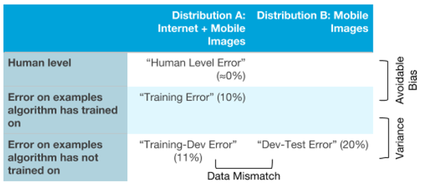
To address this, you might try to make the training data more similar to the dev/test data. It will be useful to have another dataset. Specifically, rather than giving the algorithm all the available training data, you can split it into two subsets: The actual training set which the algorithm will train on, and a separate set, which we will call the “Training dev” set, that we will not train on.
- Training set. This is the data that the algorithm will learn from.
- Training dev set: This data is drawn from the same distribution as the training set.
- Dev set: This is drawn from the same distribution as the test set, and it reflects the distribution of data that we ultimately care about doing well on.
- Test set: This is drawn from the same distribution as the dev set.
Armed with these four separate datasets, you can now evaluate:
- Training error, by evaluating on the training set.
- The algorithm’s ability to generalize to new data drawn from the training set distribution, by evaluating on the training dev set.
- The algorithm’s performance on the task you care about, by evaluating on the dev and/or test sets.
Most of the guidelines in Chapters 5-7 for picking the size of the dev set also apply to the training dev set.
41. Identifying Bias, Variance, and Data Mismatch Errors
By understanding which types of error the algorithm suffers from the most, you will be better positioned to decide whether to focus on reducing bias, reducing variance, or reducing data mismatch.
42. Addressing data mismatch
- Try to understand what properties of the data differ between the training and the dev set distributions.
- Try to find more training data that better matches the dev set examples that your algorithm has trouble with.
There is also some research on “domain adaptation” — how to train an algorithm on one distribution and have it generalize to a different distribution. These methods are typically applicable only in special types of problems and are much less widely used than the ideas described in this chapter.
Unfortunately, there are no guarantees in this process. For example, if you don’t have any way to get more training data that better match the dev set data, you might not have a clear path towards improving performance.
43. Artificial data synthesis
Keep in mind that artificial data synthesis has its challenges: it is sometimes easier to create synthetic data that appears realistic to a person than it is to create data that appears realistic to a computer.
When synthesizing data, put some thought into whether you’re really synthesizing a representative set of examples. Try to avoid giving the synthesized data properties that makes it possible for a learning algorithm to distinguish synthesized from non-synthesized examples.
Debugging inference algorithms
44. The Optimization Verification test
There are now two possibilities for what went wrong:
- Search algorithm problem.
- Objective (scoring function) problem.
In order to understand whether #1 or #2 above is the problem, you can perform the Optimization Verification test.
45. General form of Optimization Verification test
You can apply the Optimization Verification test when, given some input x, you know how to compute $ Score_{x}(y) $ that indicates how good a response y is to an input x . Furthermore, you are using an approximate algorithm to try to find arg $ max_{y} Score_{x}(y) $, but suspect that the search algorithm is sometimes failing to find the maximum.
46. Reinforcement learning example
To apply reinforcement learning, you have to develop a “Reward function” $ R(.) $ that gives a score measuring how good each possible trajectory T is.
Many machine learning applications have this “pattern” of optimizing an approximate scoring function $ Score_{x}(.) $ using an approximate search algorithm. Sometimes, there is no specified input x, so this reduces to just $ Score(.) $.
In general, so long as you have some $ y^{*} $ (in this example, $ T_{human} $ ) that is a superior output to the performance of your current learning algorithm — even if it is not the “optimal” output — then the Optimization Verification test can indicate whether it is more promising to improve the optimization algorithm or the scoring function.
End-to-end deep learning
47. The rise of end-to-end learning
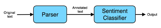
The problem of recognizing positive vs. negative opinions is called “sentiment classification”. To build this system, you might build a “pipeline” of two components:
- Parser: A system that annotates the text with information identifying the most important words.
- Sentiment classifier: A learning algorithm that takes as input the annotated text and predicts the overall sentiment.
There has been a recent trend toward replacing pipeline systems with a single learning algorithm.

Neural networks are commonly used in end-to-end learning systems. The term “end-to-end” refers to the fact that we are asking the learning algorithm to go directly from the input to the desired output.
In problems where data is abundant, end-to-end systems have been remarkably successful. But they are not always a good choice.
48. More end-to-end learning examples
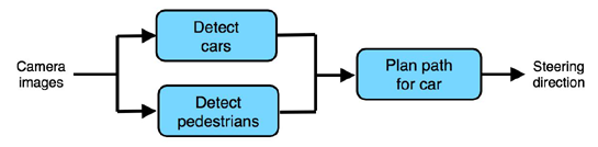
So far, we have only described machine learning “pipelines” that are completely linear: the output is sequentially passed from one staged to the next. Pipelines can be more complex. For example, here is a simple architecture for an autonomous car:
49. Pros and cons of end-to-end learning
End-to-end learning systems tend to do well when there is a lot of labeled data for “both ends” — the input end and the output end.
If you are working on a machine learning problem where the training set is very small, most of your algorithm’s knowledge will have to come from your human insight. I.e., from your “hand engineering” components. If you choose not to use an end-to-end system, you will have to decide what are the steps in your pipeline, and how they should plug together.
50. Choosing pipeline components: Data availability
One important factor for building a non-end-to-end pipeline system is whether you can easily collect data to train each of the components.
More generally, if there is a lot of data available for training “intermediate modules” of a pipeline, then you might consider using a pipeline with multiple stages. This structure could be superior because you could use all that available data to train the intermediate modules.
Until more end-to-end data becomes available, I believe the non-end-to-end approach is significantly more promising: Its architecture better matches the availability of data.
51. Choosing pipeline components: Task simplicity
Information theory has the concept of “Kolmogorov Complexity”, which says that the complexity of a learned function is the length of the shortest computer program that can produce that function. However, this theoretical concept has found few practical applications in AI. See also: https://en.wikipedia.org/wiki/Kolmogorov_complexity
If you are able to take a complex task, and break it down into simpler sub-tasks, then by coding in the steps of the sub-tasks explicitly, you are giving the algorithm prior knowledge that can help it learn a task more efficiently.
When deciding what should be the components of a pipeline, try to build a pipeline where each component is a relatively “simple” function that can therefore be learned from only a modest amount of data.
52. Directly learning rich outputs
Traditional applications of supervised learning learned a function $ h : X → Y $, where the output y was usually an integer or a real number.
One of the most exciting developments in end-to-end deep learning is that it is letting us directly learn y that are much more complex than a number.
This is an accelerating trend in deep learning: When you have the right (input,output) labeled pairs, you can sometimes learn end-to-end even when the output is a sentence, an image, audio, or other outputs that are richer than a single number.
Error analysis by parts
53. Error analysis by parts
Suppose your system is built using a complex machine learning pipeline, and you would like to improve the system’s performance. By carrying out error analysis by parts, you can try to attribute each mistake the algorithm makes to one (or sometimes both) of the two parts of the pipeline.
Our description of how you attribute error to one part of the pipeline has been informal so far: you look at the output of each of the parts and see if you can decide which one made a mistake. This informal method could be all you need.
54. Attributing error to one part
By carrying out the analysis on the misclassified dev set, you can now unambiguously attribute each error to one component. This allows you to estimate the fraction of errors due to each component of the pipeline, and therefore decide where to focus your attention.
55. General case of error attribution
The components of an ML pipeline should be ordered according to a Directed Acyclic Graph(DAG), meaning that you should be able to compute them in some fixed left-to-right order, and later components should depend only on earlier components’ outputs. Then the error analysis will be fine.
56. Error analysis by parts and comparison to human-level performance
Error analysis by parts tells us what component(s) performance is (are) worth the greatest effort to improve.
If you find that one of the components is far from human-level performance, you now have a good case to focus on improving the performance of that component.
Many error analysis processes work best when we are trying to automate something humans can do and can thus benchmark against human-level performance. If you are building an ML system where the final output or some of the intermediate components are doing things that even humans cannot do well, then some of these procedures will not apply.
57. Spotting a flawed ML pipeline
Each individual component of your ML pipeline is performing at human-level performance or near-human-level performance, but the overall pipeline falls far short of human-level. This usually means that the pipeline is flawed and needs to be redesigned. Error analysis can also help you understand if you need to redesign your pipeline.
Ultimately, if you don’t think your pipeline as a whole will achieve human-level performance, even if every individual component has human-level performance (remember that you are comparing to a human who is given the same input as the component), then the pipeline is flawed and should be redesigned.
Conclusion
58. Building a superhero team - Get your teammates to read this
The only thing better than being a superhero is being part of a superhero team. I hope you’ll give copies of this book to your friends and teammates and help create other superheroes!